A brewery that brews the right beer at the right time rarely has to dump product or scramble to fill an empty tap wall. Yet most small and mid-size breweries still plan production based on gut instinct, a whiteboard, and whatever the head brewer remembers about last summer. The result? Overproduction of slow-moving stouts in warm weather, underproduction of your flagship IPA right when demand spikes, and wasted raw materials that eat directly into margins.
The fix is straightforward, and it doesn't require a data science degree. By collecting your historical sales data, identifying seasonal patterns, and building a simple but repeatable forecasting model, you can plan production weeks or months ahead with real confidence. This guide walks you through the entire process, from gathering the right numbers to translating a forecast into a production schedule you can actually execute using a platform like BrewPlanner.
Let's get into it.
Gathering and Organizing Your Historical Sales Data
Before you can forecast anything, you need clean, reliable numbers to work with. Most breweries have sales data scattered across multiple systems: a POS for the taproom, a distributor portal for wholesale accounts, maybe a spreadsheet tracking self-distribution deliveries. The first step is pulling all of that into one place.
What Data You Actually Need
You don't need every transaction ever recorded. Focus on collecting these core data points for at least 12 months of history (24 months is better):
- Volume sold per SKU per period. Whether you measure in barrels, cases, or kegs, pick one unit and stay consistent. Break this down by week or month.
- Sales channel. Separate taproom, distribution, online, and event sales. Each channel behaves differently, and lumping them together will hide important patterns.
- Date of sale. Not the date you invoiced. Not the date you brewed. The date the product actually moved. This is the demand signal you care about.
- Price per unit at time of sale. Price changes affect volume, and you need to account for that when reading historical trends.
If you only have 6 months of data, start there. A short forecast is better than no forecast. But make a commitment to track properly from this point forward so your model gets stronger over time.
Cleaning Up the Noise
Raw sales data is messy. Before you start looking for patterns, scrub out the anomalies that would distort your forecast:
- One-time events. Did you pour 15 kegs at a beer festival that won't happen again? Flag that volume as an outlier rather than treating it as normal demand.
- Stockout periods. If your bestseller was unavailable for three weeks, sales dropped to zero during that window. But demand didn't. Estimate what you would have sold based on the weeks before and after the gap, and fill in that estimate.
- New product launches. The first month of a new release often spikes due to novelty and then settles into a steady state. Don't project that launch spike forward as the ongoing run rate.
- Bulk or contract orders. A single 50-barrel order from a festival promoter isn't recurring demand. Separate contract volume from organic demand.
A simple spreadsheet works fine for this stage. Create columns for date, SKU, channel, volume, and a flag column for outliers. Once your data is clean, you have a foundation you can trust.
Structuring Data for Analysis
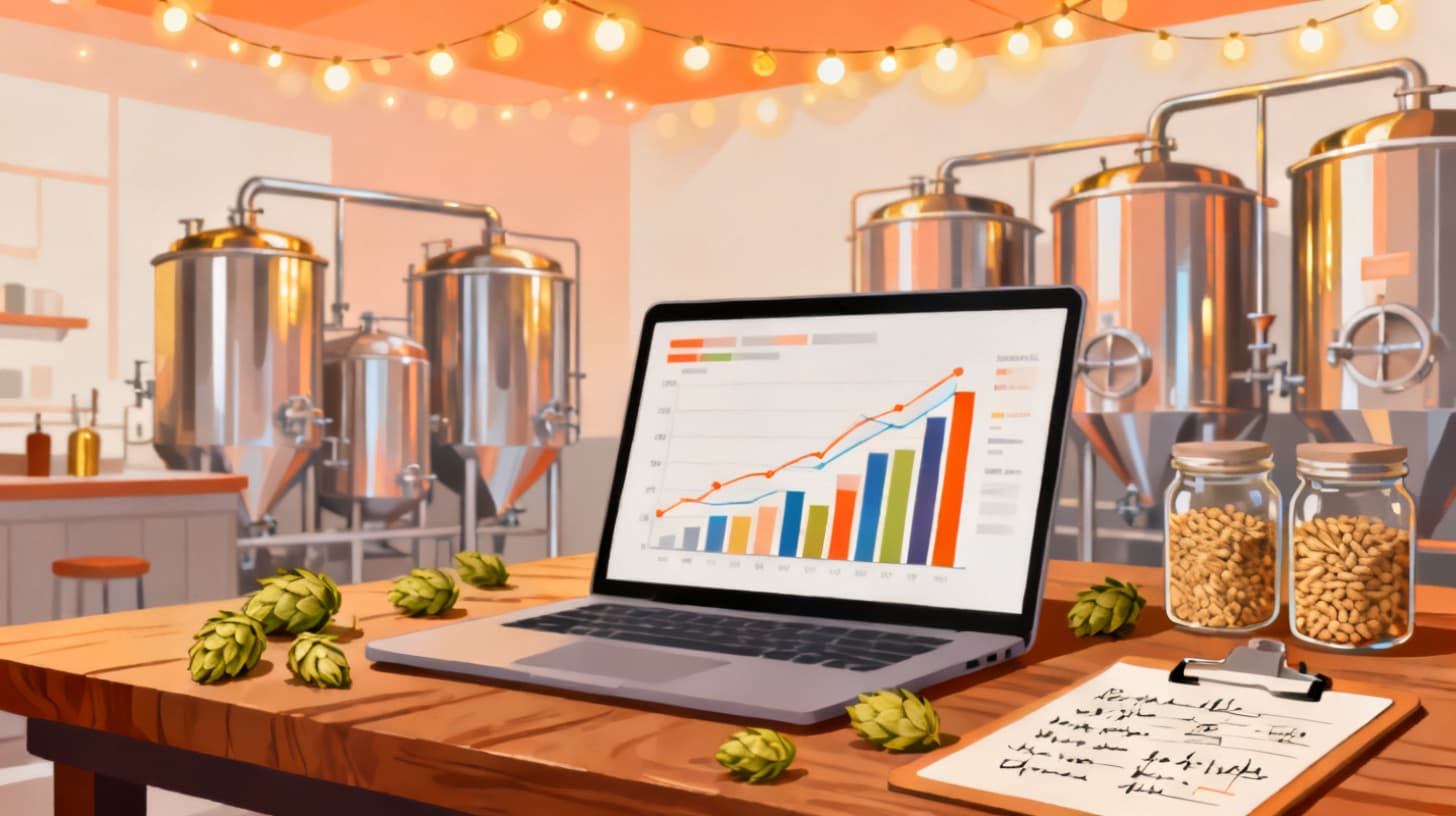
Organize your clean data into a time-series format: one row per SKU per time period (weekly or monthly), with total volume sold. This structure lets you spot trends visually before you apply any math. Build a simple line chart for each of your top 5 selling products. Even a quick glance at 12 months plotted on a graph will reveal whether a beer trends up, trends down, stays flat, or follows a wave-shaped seasonal curve.
This visual step matters more than people think. If you can see the pattern, you can forecast it. If the line looks like random noise, you may need more data or a different level of aggregation (switch from weekly to monthly, for example, to smooth out short-term volatility).
With clean, structured data in hand, you are ready to start identifying the seasonal patterns hiding inside those numbers.
Identifying Seasonal Patterns and Demand Drivers
Brewery demand is rarely random. It follows rhythms tied to weather, holidays, local events, and consumer habits. Understanding these rhythms is the core of a good forecast.
The Seasonal Index Method
The most practical tool for a brewery forecaster is the seasonal index, a simple multiplier that tells you how much higher or lower demand is in a given month compared to the annual average.
Here is how to calculate it:
- 1Calculate your average monthly sales volume for each SKU across your entire dataset. If you sold 120 barrels of Pale Ale over 12 months, your average is 10 barrels per month.
- 2For each individual month, divide actual sales by that average. If January sold 6 barrels, your January seasonal index is 0.6. If July sold 15, your July index is 1.5.
- 3If you have multiple years of data, average the indexes for each month across years. This smooths out year-specific weirdness.
Here is what a seasonal index table might look like for a fictional West Coast IPA:
MonthYear 1 Sales (bbl)Year 2 Sales (bbl)Avg SalesSeasonal IndexJan81090.69Feb911100.77Mar1113120.92Apr1315141.08May1618171.31Jun1820191.46Jul1921201.54Aug1719181.38Sep1416151.15Oct1113120.92Nov9109.50.73Dec787.50.58
The monthly average across all data is 13 barrels. Every index above 1.0 means demand is above average. Below 1.0 means below average. This single table tells you exactly when to ramp up and when to pull back.
Beyond the Calendar: External Demand Drivers
Seasonal indexes capture calendar-driven patterns, but they miss event-driven demand. Build a secondary list of recurring demand drivers specific to your market:
- Local festivals and events. If your city hosts a major music festival every summer, that is a predictable demand spike you should plan for separately.
- Holiday weekends. Memorial Day, Fourth of July, and Labor Day weekends consistently drive taproom and package sales above normal seasonal levels.
- Weather extremes. An unusually hot stretch boosts lighter, sessionable beers. A cold snap can lift stout and porter sales. While you can't predict exact weather, you can build a "weather adjustment" buffer into your forecast.
- Sports seasons. Breweries near stadiums or with strong sports-bar distribution see measurable lifts during football, baseball, or basketball seasons.
Document each driver with its approximate volume impact and expected timing. These become manual adjustments you layer on top of your seasonal index forecast.
Style-Level Seasonality
Don't just forecast at the brand level. Look at seasonality by style category too. Lighter styles (lagers, wheat beers, session IPAs) typically index high in warm months. Heavier styles (imperial stouts, barleywines, porters) index high in cold months. Flagship IPAs often maintain relatively flat demand year-round because loyal drinkers buy them regardless of season.
This style-level view helps you plan your production schedule more effectively, especially when deciding which seasonal or limited releases to slot into your calendar and when.
Building Your Forecast Model Step by Step
Now you have clean data and seasonal indexes. It is time to turn them into an actual production forecast.
Step 1: Establish Your Baseline
Your baseline is the underlying trend in your sales, stripped of seasonal fluctuation. Calculate it by dividing each month's actual sales by its seasonal index. This "de-seasonalized" number shows you whether your business is growing, shrinking, or staying flat.
For example, if your July sales were 20 barrels and July's seasonal index is 1.54, the de-seasonalized value is 20 / 1.54 = 12.99 barrels. Do this for every month, then plot those de-seasonalized values. If the line slopes upward, your business is growing. The slope tells you your monthly growth rate.
A simple way to estimate the trend: take the average de-seasonalized sales from the first half of your data and compare it to the second half. If the first half averaged 11 barrels and the second half averaged 14, you are growing at roughly 3 barrels over that span, which you can convert to a monthly growth increment.
Step 2: Project Forward
With your baseline trend and seasonal indexes, projecting forward is multiplication:
Forecasted Volume = (Baseline + Trend Growth) × Seasonal Index
Say your current de-seasonalized baseline is 14 barrels per month, your monthly growth is 0.25 barrels, and you are forecasting for April (seasonal index: 1.08). Your April forecast would be:
(14 + 0.25) × 1.08 = 15.39 barrels
Repeat for each month. Repeat for each SKU. The math is simple, but the output is powerful: a month-by-month production target for every beer in your lineup.
Step 3: Add Manual Adjustments
Layer in the external demand drivers you identified earlier. If you know a local beer festival falls in June and historically adds 5 barrels of incremental demand, add that to your June forecast. If you are planning a price increase, apply a conservative volume reduction (5-10% is a reasonable starting estimate unless you have data suggesting otherwise).
Also account for planned changes:
- New distribution accounts. If you are adding three new restaurant accounts, estimate their monthly pull based on similar existing accounts.
- Discontinued products. Remove forecasted volume for beers you are retiring, and consider whether some of that demand will shift to remaining products.
- Capacity constraints. Your forecast might say you need 25 barrels in July, but if your fermentation capacity maxes out at 20, you need to either start brewing earlier or adjust expectations.
Step 4: Convert Forecast to a Production Schedule
A demand forecast tells you what customers will buy and when. A production schedule tells you when to brew to have that product ready. The gap between them is your production lead time, which includes brewing, fermentation, conditioning, and packaging.
For a typical ale:
- Brew day: Day 0
- Fermentation: Days 1-14
- Conditioning/carbonation: Days 15-21
- Packaging: Day 22
- Available for sale: Day 23+
If your forecast says you need 15 barrels of Pale Ale available for sale by April 1, you need to start brewing by roughly March 8. Map every forecasted SKU backward through your production timeline to generate brew dates.
This is where managing your tank capacity across fermenters and brite tanks becomes critical. Your forecast might call for five different beers in production simultaneously, but if you only have three fermenters, something has to give. A visual scheduling grid lets you see conflicts before they become crises.
Step 5: Validate and Iterate
A forecast is only useful if you check it against reality. Every month, compare your forecasted volume to actual sales. Track the variance as a percentage:
Forecast Accuracy = 1 - |Actual - Forecast| / Actual
Anything above 80% accuracy is solid for a small brewery. Above 90% is excellent. When accuracy dips below 70% for a specific SKU, dig into why. Did an event you didn't anticipate drive unexpected demand? Did a competitor launch a similar product? Feed those learnings back into your model.
The forecast gets better every cycle. After three or four iterations, you will have a model that reliably predicts your production needs weeks in advance.
Turning Forecasts Into Operational Advantage
A forecast sitting in a spreadsheet is just numbers. The real payoff comes when you connect those numbers to every operational decision in your brewery.
Smarter Purchasing and Inventory
When you know how much of each beer you will brew over the next 60 to 90 days, you can order raw materials with precision. Instead of keeping 12 bags of specialty malt "just in case," you order exactly what your forecast calls for, plus a reasonable safety stock buffer of 10-15%.
This has a direct financial impact. Craft breweries typically tie up 15-25% of their working capital in raw material inventory. Reducing overstock by even 20% frees up cash you can put toward equipment, marketing, or new product development. Your forecast becomes the backbone of your purchasing schedule, and ideally feeds into an inventory management system that tracks what you have on hand against what you need.
Labor and Capacity Planning
Breweries often staff for average demand, then scramble during peaks and sit idle during valleys. Your forecast smooths this out. If you know June through August requires 40% more volume than the annual average, you can hire seasonal help in May, schedule overtime in advance, or shift some production earlier to build up packaged inventory.
The same logic applies to tank capacity. If your forecast shows three high-demand months stacking up, you can identify the bottleneck now and decide whether to brew ahead, rent temporary tank space, or contract-brew with a partner brewery.
Cash Flow and Financial Planning
Multiply your volume forecast by your average revenue per barrel, and you have a revenue forecast. Subtract your cost-per-barrel (ingredients, labor, packaging, overhead), and you have a margin forecast. This gives your finance team or your accountant a forward-looking P&L that is grounded in real production plans, not wishful thinking.
Breweries that forecast effectively can negotiate better terms with suppliers (committing to larger orders at lower prices), plan capital expenditures around cash-rich periods, and avoid the feast-or-famine cash cycles that sink so many small producers.
Bringing It All Together
The most effective breweries don't treat forecasting as a one-time exercise. They build it into a monthly planning rhythm:
- Pull last month's actual sales by SKU and channel
- Compare actuals to forecast and log variances
- Update seasonal indexes if new data reveals shifting patterns
- Re-run the forecast for the next 90 days
- Convert the updated forecast to a brew schedule
- Align purchasing, staffing, and tank allocation to the new plan
This cycle takes a few hours per month once you have the framework built. The return is a brewery that operates proactively instead of reactively, that wastes less, sells more, and runs leaner.
If you are ready to connect your demand forecast to a production scheduling system that manages orders, tank assignments, and inventory in one place, BrewPlanner is built for exactly this workflow. It gives you the visual dashboard and operational tools to turn your forecast numbers into an executed production plan, without the spreadsheet chaos.
Start with the data you have. Build the simplest version of this model. Refine it every month. Within a few cycles, you will wonder how you ever brewed without it.